2 Variations
2.1 How many variations are included in the dataset?
There are 4,156,427 SNPs (single nucleotide polymorphisms) and 1,442,744 InDels (inserts and deletions) identified using the whole dataset in our study.
2.2 How the variations are identified?
Leaves were collected from plants in vegetative growth phase in the field for each accession and genomic DNA was then extracted from the fresh leaf tissue using DNeasy Plant Mini Kit (Qiagen). A sequencing library with ~400bps (base pairs) insert size was constructed by Trueprep Tagment 3 Enzyme (Tn5 transposase, Vazyme). The amplification-free method for library construction was used in our work in order to accurately judge heterozygous sites by reducing duplicate sequences. Sequencing was performed on the NovaSeq 6000 platform with average coverage 35×, generating 150bps paired-end reads. Quality control was conducted for the paired-end raw reads using the software Trimmomatic (version 0.38)(Bolger et al., 2014), and bases of low quality or from adapter contamination were removed by the trimming tools with parameters “ILLUMINACLIP:TruSeq3-PE.fa:2:30:10:2:true MAXINFO:50:0.6”. The clean reads were then aligned against the rice reference genome IRGSP1.0 by software BWA (version 0.7.1)(Li et al., 2010) with parameters of “-R “@RG:SampleID:Illumina:SampleName” -M”. Read alignment results were sorted according to their coordination by “SortSam” and duplicated reads were marked by “MarkDuplicates” functions in GATK (the genome analysis toolkit v4.1.4.1)(McKenna et al., 2010) with default parameters. Variations were called using “HaplotypeCaller”, “GenomicsDBImport” and “GenotypeGVCFs” functions in GATK. High quality variations were further identified with the “VariantFiltration” function in GATK with parameters of “–cluster-size 3 –cluster-window-size 10 QD < 10.00 FS > 15.000 AC < 3 DP>200||DP<5” for SNPs and “QD<10.00 FS>30.000 DP>200||DP<5” for InDels.
2.3 How to search variations?
Users can get access to variation information by clicking the “Variant Search” or “Variants” button on the navigation bar (as shown in Figure2.1).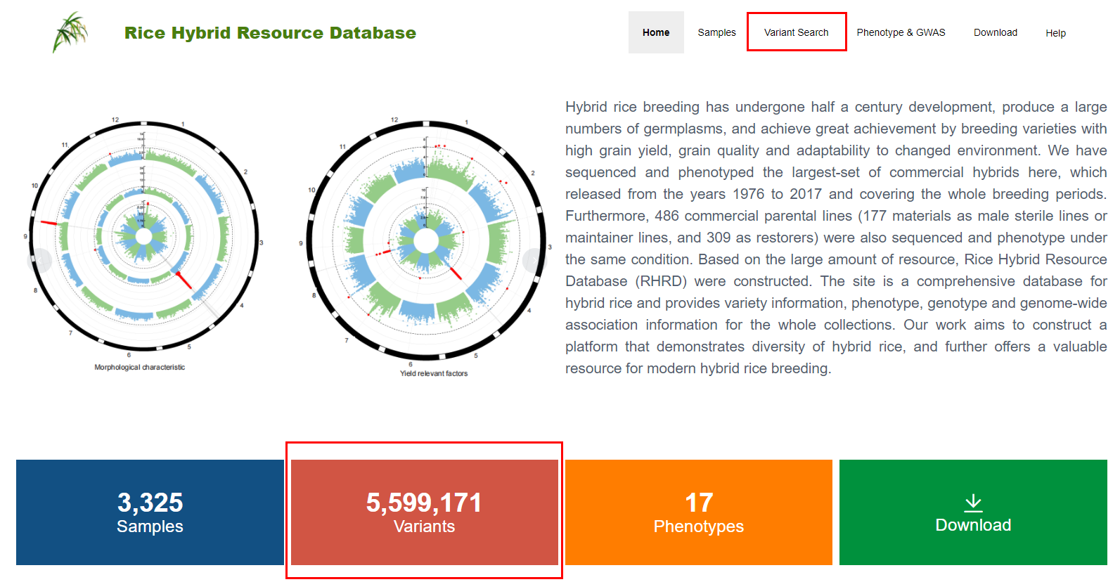
Figure 2.1: The navigation bar on the home page
Dataset, population and specify genomic region by chromosome, start and end (Figure2.2), or by gene ID (Figure2.3). The genomic region should be less than 10,000 base pairs when users specify the genomic region by chromosome, start and end.
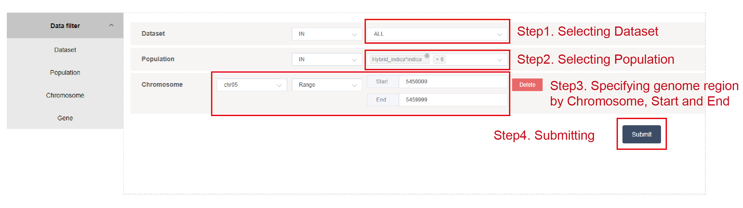
Figure 2.2: Specifying genomic region by Chromosome, Start and End
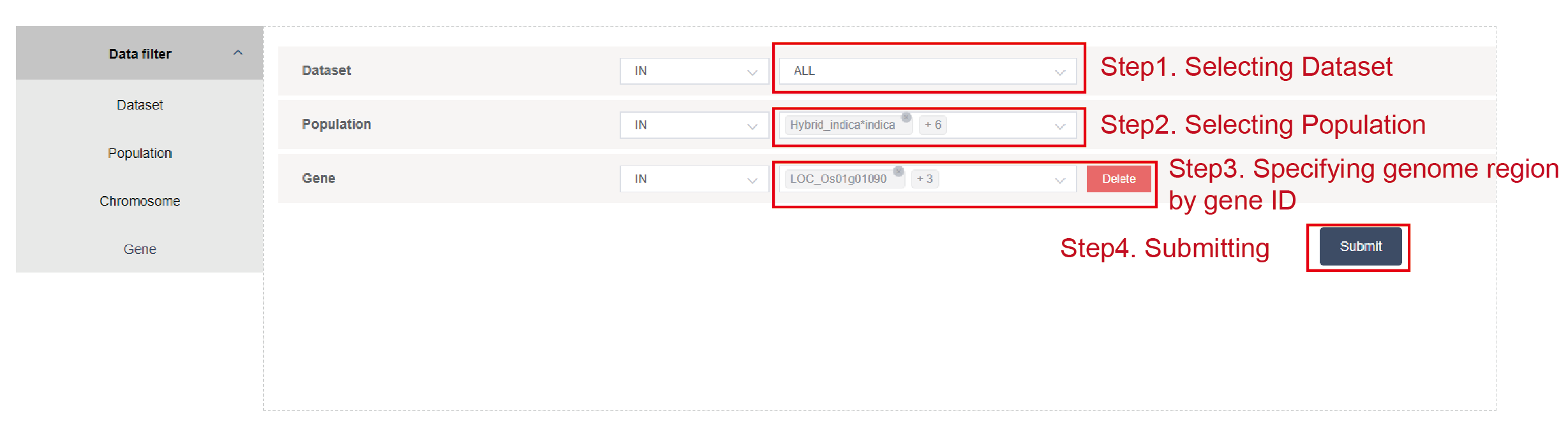
Figure 2.3: Specifying genomic region by gene ID
2.4 Overview the composition of the “Variant” page
The “variant” page consists of 4 parts:
2.4.1 Annotation of variations in the target region from selected samples
We use software SnpEff (v 4.3t) (Cingolani et al., 2012) to do variation annotation and demonstrate the potential impact of variants. The gene model (snpEff_v4_3_ENSEMBL_BFMPP_32_268.zip) is used for annotation. We demonstrate and color the variants based on their putative impacts estimated by SnpEff. Based on SnpEff, there are 4 putative impacts for variants.
High
The variant is assumed to have high (disruptive) impact in the protein, probably causing protein truncation, loss of function or triggering nonsense mediated decay.
Moderate
A non-disruptive variant that might change protein effectiveness.
Low
Assumed to be mostly harmless or unlikely to change protein behavior.
Modifier
Usually non-coding variants or variants affecting non-coding genes, where predictions are difficult or there is no evidence of impact.
The proportion of four types of variants leading to different impacts is shown by pieplot on the top of the page. Furthermore, the SnpEff also indicates the feature type of variants, for example the “upstream gene variant”, “downstream gene variant”, “nonsynonymous variant” and so on, and assign the putative impact for each type of feature. The proportion of different feature types for variants leading to the same impact is also demonstrated (Figure2.4). For each component in pieplot, users can hide it by pressing the component in figure legends (Figure2.5).
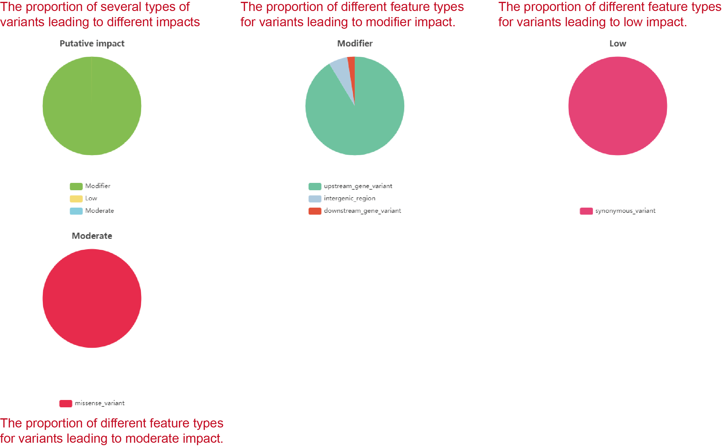
Figure 2.4: Annotation of variations in the target region from selected samples
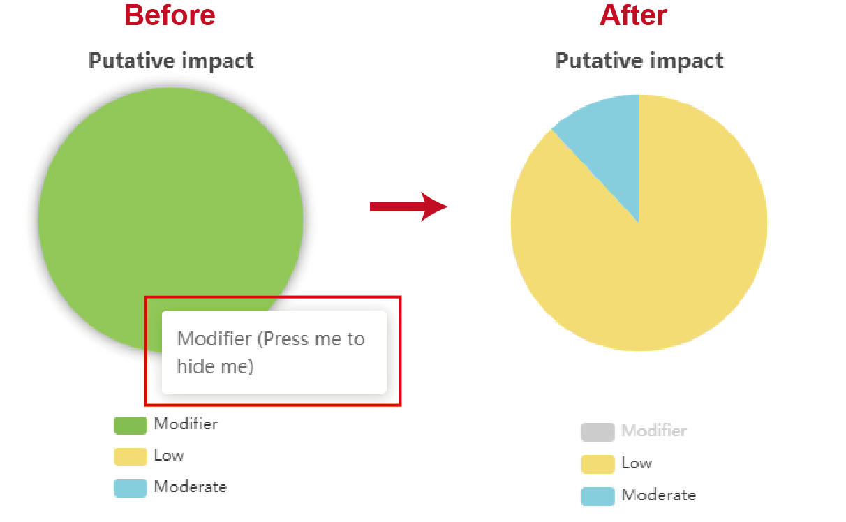
Figure 2.5: Hiding a component by pressing it in figure legends
2.4.2 Allelic information for variations from target region in seleted samples
Following the overview of variant annotation, a table lists detailed allelic information for all variants from target region in selected samples. And the alleles are colored according to their putative impact, corresponding with that in “annotation” part. The missing data are represented by symbol “.”.
Note
User can drag and drop the scroll bar below the table to view all the variants in target region
User can go to any page by providing page number to view the information in all samples.
User can customize the number of variants displayed on each page.
User can get access to any sample quickly by searching for sample ID.
User can place cursor to show complete information for any cell in the table.
The download button is provided on the top of the table.
Seeing Figure2.6 for details.
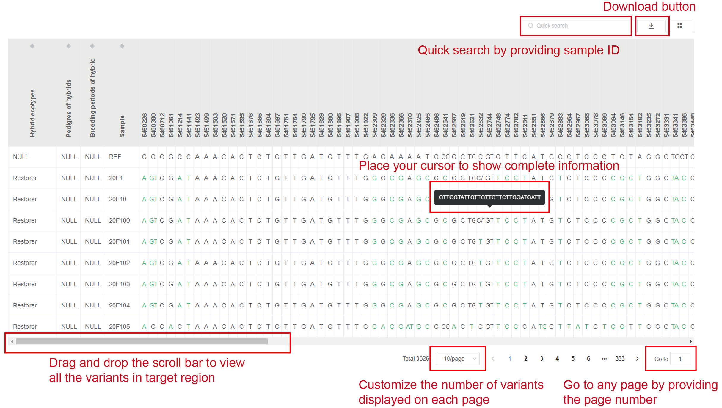
Figure 2.6: Details of allelic information
2.4.3 Allelic frequency of each site from target region among selected subpopulations
Below the table, we calculate and demonstrate the allelic frequency for each site from target region among the selected subpopulation. Users can select desired variants by dragging the bar below the figure. Users can get access to details by placing the cursor on the interested site.
2.4.4 Haplotype analysis
Users can conduct haplotype analysis for selected sites. All sites in target region are listed in selection window. Users can click the desired sites to pick on them (Figure2.7), and can also drag their mouse to chose multiple sites each time (Figure2.8). Multiple selections could be accumulated.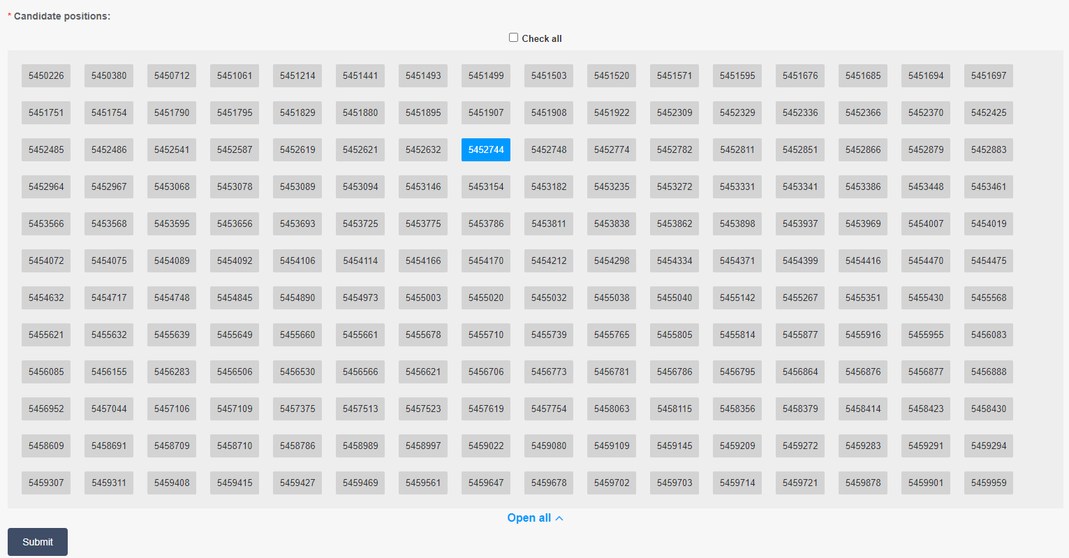
Figure 2.7: Pressing desired site to pick on it
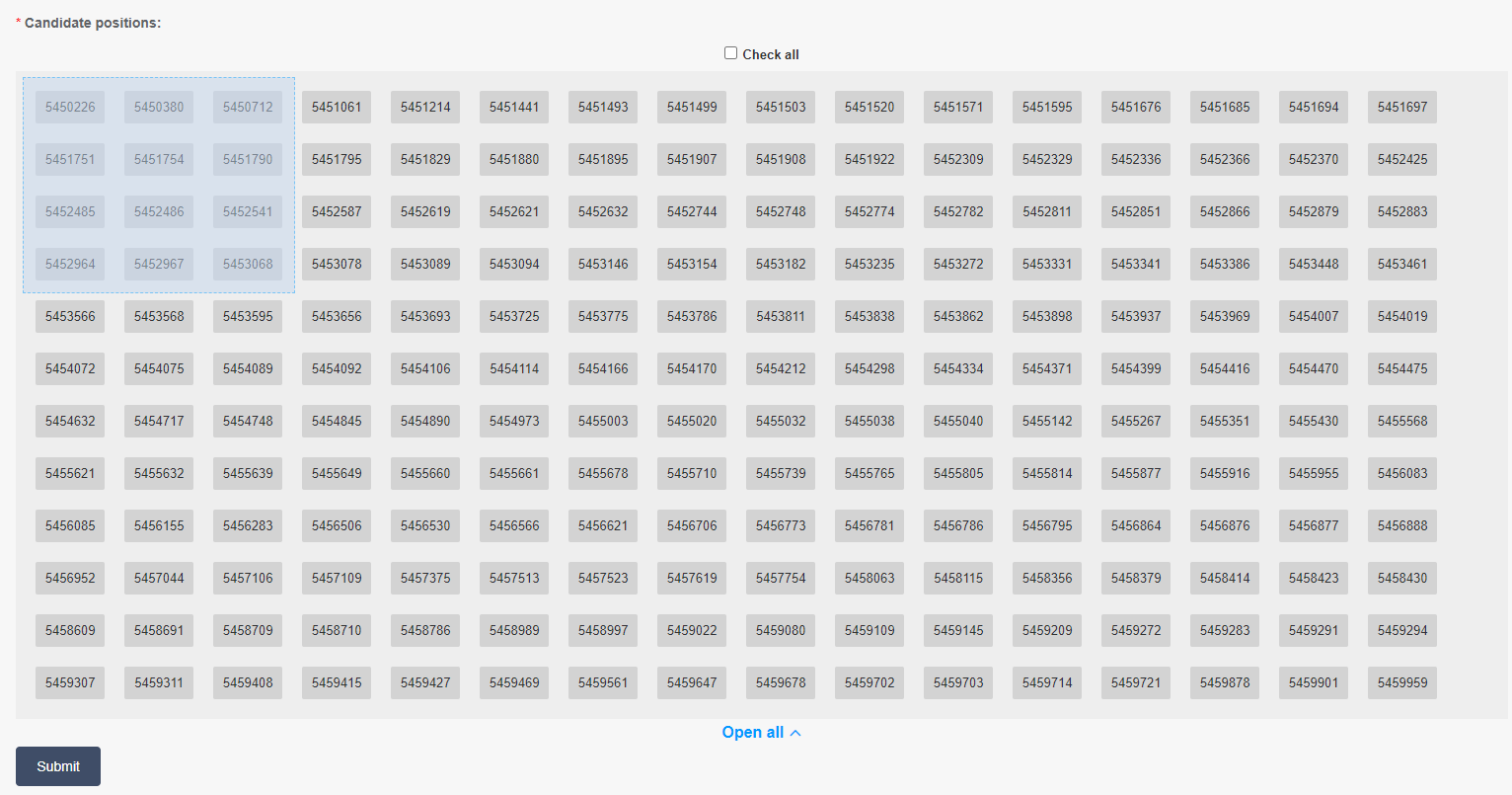
Figure 2.8: dragging to chose multiple sites
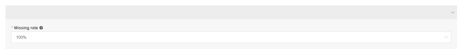
Figure 2.9: Filtering sites with missing rate
After submitting, the results are displayed below. The proportions of all haplotypes within selected subpopulations are shown by pieplot. Details for haplotype information are listed in a table, including the genotype of all haplotypes and sample composition of each haplotype.
2.5 Reference
Bolger, A.M., Lohse, M. & Usadel, B. Trimmomatic: a flexible trimmer for Illumina sequence data. Bioinformatics 30, 2114-2120 (2014).
Li, H. & Durbin, R. Fast and accurate long-read alignment with Burrows-Wheeler transform. Bioinformatics 26, 589-595 (2010).
McKenna, A. et al. The Genome Analysis Toolkit: a MapReduce framework for analyzing next-generation DNA sequencing data. Genome Res 20, 1297-1303 (2010).
Cingolani, P. et al. A program for annotating and predicting the effects of single nucleotide polymorphisms, SnpEff: SNPs in the genome of Drosophila melanogaster strain w1118; iso-2; iso-3. Fly 6, 1-13 (2012).